Color model – Core Flooding
The core flooding protocol is designed to mimic SCAL experiments where one immiscible fluid is injected into the sample at a constant rate, displacing the other fluid. The core flooding protocol relies on a flux boundary condition to ensure that fluid is injected into the sample at a constant rate. The flux boundary condition implements a time-varying pressure boundary condition that adapts to ensure a constant volumetric flux. Details for the flux boundary condition are available (see: https://doi.org/10.1016/j.compfluid.2020.104670)
protocol = "core flooding"
To match experimental conditions, it is usually important to match the capillary number, which is

where  is the dynamic viscosity,
  is the fluid
(usually water) velocity and
is the fluid
(usually water) velocity and  is the interfacial tension.
The volumetric flow rate is related to the fluid velocity based on
is the interfacial tension.
The volumetric flow rate is related to the fluid velocity based on

where  is the cross-sectional area and
  is the porosity. Given a particular experimental system
self-similar conditions can be determined for the lattice Boltzmann
simulation by matching the non-dimensional
is the porosity. Given a particular experimental system
self-similar conditions can be determined for the lattice Boltzmann
simulation by matching the non-dimensional  . It is nearly
awlays advantageous for the timestep to be as large as possible so
that time-to-solution will be more favorable. This is accomplished by
. It is nearly
awlays advantageous for the timestep to be as large as possible so
that time-to-solution will be more favorable. This is accomplished by
use a high value for the numerical surface tension (e.g.
alpha=1.0e-2)use a small value for the fluid viscosity (e.g.
tau_w = 0.7andtau_n = 0.7)determine the volumetric flow rate needed to match
For the color LBM the interfacial tension is
 and the dynamic viscosity is
 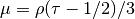 ,
where the units are relative to the lattice spacing, timestep and mass
density. Agreemetn between the experimental and simulated values for
is ensured by setting the volumetric flux
,
where the units are relative to the lattice spacing, timestep and mass
density. Agreemetn between the experimental and simulated values for
is ensured by setting the volumetric flux
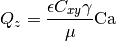
where the LB units of the volumetric flux will be voxels per timestep.
In some situations it may also be important to match other non-dimensional numbers, such as the viscosity ratio, density ratio, and/or Ohnesorge/Laplace number. This can be accomplished with an analogous procedure. Enforcing additional constraints will necessarily restrict the LB parameters that can be used, which are ultimately manifested as a constraint on the size of a timestep.
Color {
   protocol = "core flooding"
   capillary_number = 1e-4            // capillary number for the displacement
   timestepMax = 1000000              // maximum timtestep
   alpha = 0.005                      // controls interfacial tension
   rhoA = 1.0                         // controls the density of fluid A
   rhoB = 1.0                         // controls the density of fluid B
   tauA = 0.7                         // controls the viscosity of fluid A
   tauB = 0.7                         // controls the viscosity of fluid B
   F = 0, 0, 0                        // body force
   WettingConvention = "SCAL"         // convention for sign of wetting affinity
   ComponentLabels = 0, -1, -2        // image labels for solid voxels
   ComponentAffinity = 1.0, 1.0, 0.6  // controls the wetting affinity for each label
   Restart = false
}
Domain {
   Filename = "Bentheimer_LB_sim_intermediate_oil_wet_Sw_0p37.raw"
   ReadType = "8bit"              // data type
   N = 900, 900, 1600             // size of original image
   nproc = 2, 2, 2                // process grid
   n = 200, 200, 200              // sub-domain size
   offset = 300, 300, 300         // offset to read sub-domain
   voxel_length = 1.66            // voxel length (in microns)
   ReadValues = -2, -1, 0, 1, 2   // labels within the original image
   WriteValues = -2, -1, 0, 1, 2  // associated labels to be used by LBPM
   BC = 4                         // boundary condition type (0 for periodic)
}
Analysis {
   analysis_interval = 1000           // logging interval for timelog.csv
   subphase_analysis_interval = 5000  // loggging interval for subphase.csv
   visualization_interval = 100000    // interval to write visualization files
   N_threads = 4                      // number of analysis threads (GPU version only)
   restart_interval = 1000000         // interval to write restart file
   restart_file = "Restart"           // base name of restart file
}
Visualization {
   write_silo = true     // write SILO databases with assigned variables
   save_8bit_raw = true  // write labeled 8-bit binary files with phase assignments
   save_phase_field = true  // save phase field within SILO database
   save_pressure = false    // save pressure field within SILO database
   save_velocity = false    // save velocity field within SILO database
}
FlowAdaptor {
}