Color model – Centrifuge Protocol¶

The centrifuge protocol is designed to mimic SCAL centrifuge experiments that are used to infer the capillary pressure. The LBPM centrifuge protocol is constructed as an unsteady simulation with constant pressure boundary conditions and zero pressure drop across the sample. This will enforce the following key values

BC = 3 – constant pressure boundary condition
din = 1.0 – inlet pressure value
dout = 1.0 – outlet pressure value

By default LBPM will populate the inlet reservoir with fluid A (usually the non-wetting fluid) and the outlet reservoir with fluid B (usually water). Flow is induced by setting an external body force to generate displacement in the z direction. If the body force is set to zero, e.g. F = 0, 0, 0, the simulation will produce spontaneous imbibition, with the balancing point being determined based on zero pressure drop across the sample. Setting an external body force will shift the capillary pressure. Setting a positive force will cause fluid A to be forced into the sample. Once steady conditions are achieved, the pressure of fluid A will be larger than fluid B. Alternatively, if the driving force is negative then fluid B will be forced into the sample, and the steady-state configuration will stabilize to a configuration where fluid B has a larger pressure compared to fluid A. The capillary pressure is thereby inferred based on the body force.

In a conventional SCAL experiment the centrifugal forces are proportional to the density difference between fluids. While this is still true for LBPM simulation, the body force will still be effective even if there is no difference in density between the fluids. This is because a positive body force will favor a larger saturation of fluid A (positive capillary pressure ) whereas a negative body force will favor a lower saturation of fluid A (negative capillary pressure).

The simplest way to infer the capillary pressure is based on consideration of the average fluid pressures, which are logged to the output files timelog.csv and subphase.csv. In the units of the lattice Boltzmann simulation, the interfacial tension is given as $\gamma_{wn} = 6 \alpha$ . Suppose that the physical interfacial tension is given by $\gamma_{wn}^\prime$ , provided in units of Pa-m. The capillary pressure in pascal will then be given by

$p_c^\prime = \frac{\gamma_{wn}^\prime (p_n - p_w)}{\gamma_{wn} \Delta x}$

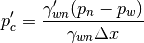
where $\Delta x$ is the voxel length in meters.

To enable the centrifuge protocol such that the effective pressure of fluid B is higher than fluid A, the input file can be specified as below. Increasing the body force will lead to a larger capillary pressure.

Color {
   protocol = "centrifuge"
   timestepMax = 1000000              // maximum timtestep
   alpha = 0.005                      // controls interfacial tension
   rhoA = 1.0                         // controls the density of fluid A
   rhoB = 1.0                         // controls the density of fluid B
   tauA = 0.7                         // controls the viscosity of fluid A
   tauB = 0.7                         // controls the viscosity of fluid B
   F = 0, 0, -1.0e-5                  // body force
   din = 1.0                          // inlet density (controls pressure)
   dout = 1.0                         // outlet density (controls pressure)
   WettingConvention = "SCAL"         // convention for sign of wetting affinity
   ComponentLabels = 0, -1, -2        // image labels for solid voxels
   ComponentAffinity = 1.0, 1.0, 0.6  // controls the wetting affinity for each label
   Restart = false
}
Domain {
   Filename = "Bentheimer_LB_sim_intermediate_oil_wet_Sw_0p37.raw"
   ReadType = "8bit"              // data type
   N = 900, 900, 1600             // size of original image
   nproc = 2, 2, 2                // process grid
   n = 200, 200, 200              // sub-domain size
   offset = 300, 300, 300         // offset to read sub-domain
   voxel_length = 1.66            // voxel length (in microns)
   ReadValues = -2, -1, 0, 1, 2   // labels within the original image
   WriteValues = -2, -1, 0, 1, 2  // associated labels to be used by LBPM
   BC = 3                         // boundary condition type (0 for periodic)
}
Analysis {
   analysis_interval = 1000           // logging interval for timelog.csv
   subphase_analysis_interval = 5000  // loggging interval for subphase.csv
   visualization_interval = 100000    // interval to write visualization files
   N_threads = 4                      // number of analysis threads (GPU version only)
   restart_interval = 1000000         // interval to write restart file
   restart_file = "Restart"           // base name of restart file
}
Visualization {
   write_silo = true     // write SILO databases with assigned variables
   save_8bit_raw = true  // write labeled 8-bit binary files with phase assignments
   save_phase_field = true  // save phase field within SILO database
   save_pressure = false    // save pressure field within SILO database
   save_velocity = false    // save velocity field within SILO database
}
FlowAdaptor {
}